← Live courses
LiveEnglishIntermediateZoomAI agentsExcel + iziRisk Quantum

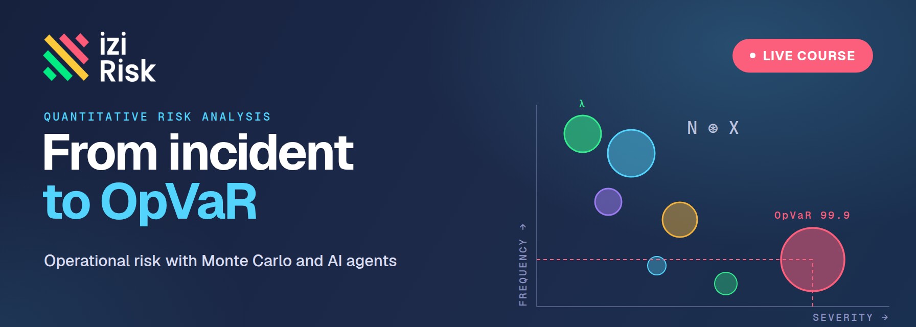
Operational risk quantification: from the loss-event database to OpVaR with Monte Carlo and AI agents

With Fernando Hernández. Six two-hour sessions to turn a financial institution’s loss-event database into an annual loss distribution by event type, with frequency and severity fitted and convolved, and to calculate OpVaR, expected shortfall and the capital each event type consumes.

  1. Mon30Nov
  2. Wed2Dec
  3. Mon7Dec
  4. Wed9Dec
  5. Mon14Dec
  6. Wed16Dec
6 sessions · 12 hours12:00–14:00 New York · 17:00–19:00 London · 09:00–11:00 Los Angeles
  • ✓ 6 live sessions on Zoom, and their recordings
  • ✓ 3 months of the Professional licence: the operational-risk model with your own loss database, the AI agents, the iziRisk Quantum Excel add-in and the downloadable materials · What's in it?
  • ✓ The “Operational risks for financial institutions” Excel workbook (professional version) and the 1,500-event demo register, in five languages

US$240US$340

Launch price until 19 November

By the end you will be able to

  • ✓Explain the loss distribution approach (LDA): why annual operational loss is a random variable, and how expected loss, unexpected loss and OpVaR differ.
  • ✓Organise and clean a loss-event database with the three-level Basel classification, gross loss, recovery and net loss, and measure the observation window correctly.
  • ✓Model the frequency of each event type with a Poisson or negative binomial, and recognise overdispersion in the monthly counts.
  • ✓Fit severity with the lognormal by moments and by maximum likelihood, the gamma, the Weibull or the empirical distribution, and choose with the Kolmogorov–Smirnov distance and the S-curve, paying special attention to the tail.
  • ✓Convolve frequency and severity with Monte Carlo, correlate the event types from their monthly losses and measure the diversification benefit.
  • ✓Calculate OpVaR at 99.9%, unexpected loss and expected shortfall (ES), and allocate capital across event types by their contribution to the worst years.
  • ✓Read and interpret histograms, S-curves, exceedance curves, the risk horizon and a multi-year loss horizon checked against history, and reproduce the model in Excel with iziRisk Quantum and izConvolute.
  • ✓Work with the AI agent that interprets the results and drafts the report for the risk committee, and review what it proposes with judgement.

Who it is for

Operational risk managers and analysts, internal control, compliance, internal audit, model validation and supervisors at banks, insurers, cooperatives, microfinance institutions and fintechs. Also insurance teams who assess operational risk cover.

Prerequisites

Intermediate Excel and familiarity with an incident or loss-event register. No advanced statistics or programming needed.

Includes

  • 6 live sessions on Zoom, and their recordings.
  • 3 months of the Professional licence: the operational-risk model with your own loss database, the AI agents, the iziRisk Quantum Excel add-in and the downloadable materials.
    › What's in it?

    Operational risk model (LDA)

    • Your own loss-event database, in any language, with Basel codes or your own categories, not just the demo register (locked on the Student account).
    • Event types correlated from their monthly losses or at a uniform level (locked on the Student account).
    • Simulations of up to 200,000 iterations, against 200 on the Student account.
    • Frequency and severity fitting by event type, with the Kolmogorov–Smirnov distance and the S-curve of each fit.
    • Export of the model to Excel (.xlsm) with izConvolute, and a PDF report with charts and analysis.

    AI agents

    • Analyse every simulation and explain it in plain language for the risk committee: where the capital sits, how far to trust each fit and where to act.
    • Build Excel Monte Carlo models and turn a deterministic Excel model into a probabilistic one (“Just iziRisk it!”).
    • Generous use: over a hundred analyses a month, against a few in total on the Student account.

    Excel and materials

    • The iziRisk Quantum Excel add-in with up to 50,000 iterations per simulation, distribution fitting and a correlation matrix.
    • Unlimited downloads of course materials: PDFs, workbooks and resources.

    Experts

    • The “Ask the Expert” AI chat, answered from indexed expert content.
    • Up to 30 questions a month to human experts.
    See the full Professional plan →
  • The “Operational risks for financial institutions” Excel workbook (professional version) and the 1,500-event demo register, in five languages.
  • Certificate of 12 hours of training.

Minimum 8, maximum 25 participants.
Dates and times · 6 sessions, 12 hours

  1. SESSION 1

    Monday 30 November

    12:00–14:00 New York

    Operational loss is a distribution: the LDA approach

    An institution does not lose its average loss every year: it loses through many small events and, now and then, through one that is not forgotten. The loss distribution approach describes both at once — how many events and how much each one costs — and OpVaR and capital come from that distribution.

    • What an operational loss event is: date, gross loss, recovery, net loss and cause.
    • The Basel classification: seven event types on three levels, and the cause families (people, processes, systems and external events).
    • Expected loss, unexpected loss, OpVaR at 99.9% and expected shortfall.
    • What LDA is for today: economic capital, ICAAP, risk appetite and management, alongside the regulatory standardised approach.
    • What iziRisk’s AI agents do in operational risk analysis.

    Hands-on: Load the 1,500-event demo register, run the first simulation and read the annual loss distribution.

  2. SESSION 2

    Wednesday 2 December

    12:00–14:00 New York

    The loss-event database and frequency

    • Column mapping, Basel codes and derived levels; categories such as unit, cause or product.
    • Data quality: collection thresholds, recoveries, misclassified events and how to spot them.
    • The observation window: λ = events ÷ years observed, and how wrong a fixed divisor gets it.
    • Exploratory analysis: monthly series, the heat map by event type and unit, and the largest events.
    • Frequency with the Poisson and the negative binomial: the variance-to-mean ratio of monthly counts and the dispersion k.

    Hands-on: Analyse the register, find its concentrations and choose between Poisson and negative binomial for each event type.

  3. SESSION 3

    Monday 7 December

    12:00–14:00 New York

    Severity: fitting the distribution of each loss

    Operational capital is set by the tail of the severity: the rare, large events. Different families can describe the middle of the data equally well and differ by a factor of two at the 99.9th percentile. This session teaches how to choose on evidence and to distrust the tail.

    • The lognormal by moments (the workbook’s izLogNormal) against maximum likelihood; gamma and Weibull.
    • The empirical distribution: why it can never produce a loss larger than the largest on record.
    • Goodness of fit: the Kolmogorov–Smirnov distance and the S-curve on a log scale.
    • Cells with few events, heavy tails and the choice of Basel level: homogeneity against data.

    Hands-on: Fit the severity of each level-2 event type, choose the family on evidence and measure the effect of that choice on OpVaR.

  4. SESSION 4

    Wednesday 9 December

    12:00–14:00 New York

    Convolution, correlation and capital

    • Frequency ⊛ severity convolution with Monte Carlo: one year per iteration, and izConvolute in Excel.
    • Iterations, Latin Hypercube and how many years lie beyond the 99.9th percentile.
    • Correlation between event types from their monthly losses, with Iman–Conover; the diversification benefit and why the independence assumption exaggerates it.
    • Standalone versus capital allocated by contribution to the tail; what drives the total.
    • The risk horizon: frequent and cheap against rare and ruinous.

    Hands-on: Simulate the register with and without correlations and explain the effect on OpVaR, expected shortfall and the capital allocation.

  5. SESSION 5

    Monday 14 December

    12:00–14:00 New York

    Reports and the model in Excel with iziRisk Quantum

    • Histograms, S-curves and exceedance curves: from the 1-in-20-year loss to the 1-in-1,000.
    • The multi-year loss horizon and the test against the register’s own history.
    • From the web model to the .xlsm workbook: the Model, Losses and Ref sheets, and izConvolute(izPoisson, izLogNormal).
    • Inputs, outputs and correlations already declared: simulate in Excel and reconcile with the web model.
    • Adapting the workbook to your own loss database.

    Hands-on: Export the model, simulate it in Excel and reconcile expected loss, OpVaR and capital with the web model.

  6. SESSION 6

    Wednesday 16 December

    12:00–14:00 New York

    Validating, deciding and presenting to the risk committee

    • Validation: expected loss against history, stability across seeds, sensitivity to the window, the threshold and the severity family.
    • Scenarios and stress: more events, more severe events and what happens to capital.
    • Deciding with the model: controls for frequent event types, insurance and risk transfer for severe ones.
    • What to report to the committee, what not to, and how to tell it to the person who decides. The AI agent that analyses the simulation and the PDF report, without handing it the judgement.
    • Clinic: volunteers present their loss database and get feedback. Wrap-up and certificates.

    Hands-on: The one-page report for the risk committee on your own loss database or the demo register.

Ask a question